There are several things you should be aware of while analyzing NHANES data with Stata. Please see the Stata Tips page to review them before continuing.
In this example, you will use Stata to generate tables of means and standard errors for average cholesterol levels of persons 20 years and older by sex and race-ethnicity. Following that example, is an example of calculating the geometric means.
There are several things you should be aware of while analyzing NHANES data with Stata. Please see the Stata Tips page to review them before continuing.
Remember that you need to define the SVYSET before using the SVY series of commands. The general format of this command is below:
svyset [w=weightvar], psu(psuvar) strata(stratavar) vce(linearized)
To define the svyset for your cholesterol analysis, use the weight variable for four-yours of MEC data (wtmec4yr), the PSU variable (sdmvpsu), and strata variable (sdmvstra) .The vce option specifies the method for calculating the variance and the default is "linearized" which is Taylor linearization. Here is the svyset command for four years of MEC data:
svyset [w= wtmec4yr], psu( sdmvpsu) strata(sdmvstra) vce(linearized)
Now, that the svyset has been defined you can use the Stata command, svy: mean, to generate means and standard errors. The general command for obtaining weighted means and standard errors of a subpopulation is below.
svy: mean varname, subpop(if condition)
Here is the command to generate the mean cholesterol (lbxtc) for the subpopulation of adults over the age of 20 (ridageyr>=20 & ridageyr <.):
svy: mean lbxtc, subpop(if ridageyr >=20 & ridageyr <. )

You can also add the over() option to the svy:mean command to generate the means for different subgroups. When you do this, you can type a second command, estat size, to have the output display the subgroup observation numbers. Here is the general format of these commands for this example:
svy: mean varname, subpop(if condition) over(var1 var2)
estat size
The prefix quietly before any svy command suppresses the appearance of the output of a command on the screen. In the following example, the first command is done "quietly"; the second command is executed to show the mean, standard error, plus the number of observations in each category. Below is the command to generate the mean cholesterol (lbxtc) for the subpopulation of adults over the age of 20 (ridageyr>=20 & ridageyr <.) by gender (riagendr).
quietly svy: mean lbxtc, subpop(if ridageyr>=20 & ridageyr <. ) over(riagendr)
estat size

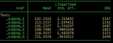
Additionally, the over option can take multiple variables. To generate means for the six gender-age groups you will need to add the age variable to the over option, as in the example below.
quietly svy: mean lbxtc, subpop(if ridageyr>=20 & ridageyr <. ) over(riagendr age)
estat size

The output will list the sample sizes, means, and their standard errors for each of the six gender-age groups.
If you need to generate geometric means instead of arithmetic means, you would first log transform the variable of interest. Then, use the svy:mean command to obtain the mean of the transformed variable. Finally, display the exponentiated form of the variable. The general format of these commands is:
generate ln_varname=ln(varname)
quietly svy: mean ln_varname, subpop(if condition) over(var1)
ereturn display, eform(geo_mean)
To generate geometric means of the cholesterol variable for persons aged 20 years and older by gender using the previous dataset, you would need to run the following commands and options.
The example below is for illustrative purposes only. Geometric means are not recommended for use with normally distributed data, such as the cholesterol variables in this dataset.
First, create a new variable which is equal to the natural log of the variable of interest. In this example, the variable of interest is the cholesterol variable (lbxtc).
generate ln_lbxtc=ln(lbxtc)
Then, estimate the mean of the log transformed cholesterol variable (ln_lbxtc) for persons over the age of 20 (ridageyr>=20 & ridageyr <.) by gender (riagendr). The quietly prefix is used to suppress the output.
quietly svy: mean ln_lbxtc, subpop(if ridageyr>=20 & ridageyr <. ) over(riagendr)
Finally, display the output in original units. Stata lets you do this automatically by using the command eform(geo_mean), which displays the exponentiated coefficients for the mean, standard error, and 95% CI (ie, it calculates e to the (ln_lbxtc) power.
ereturn display, eform(geo_mean)