There are several things you should be aware of while analyzing NHANES data with Stata. Please see the Stata Tips page to review them before continuing.
In this task, you will use the chi-square test in Stata to determine whether gender and blood pressure cuff size are independent of each other. The chi-square statistics is requested from the Stata command svy:tabulate.
There are several things you should be aware of while analyzing NHANES data with Stata. Please see the Stata Tips page to review them before continuing.
Remember that you need to define the SVYSET before using the SVY series of commands. The general format of this command is below:
svyset [w=weightvar], psu(psuvar) strata(stratavar) vce(linearized)
To define the survey design variables for your blood pressure cuff size (bpacsz) analysis, use the weight variable for four-yours of MEC data (wtmec4yr), the PSU variable (sdmvpsu), and strata variable (sdmvstra) .The vce option specifies the method for calculating the variance and the default is "linearized" which is Taylor linearization. Here is the svyset command for four years of MEC data:
svyset [w= wtmec4yr], psu(sdmvpsu) strata(sdmvstra) vce(linearized)
In this example, a new variable (cuff_size) is created to regroup blood pressure cuff size (bpacsz) from five categories to four categories. This collapses the infant (1) and child (2) groups. Use the gen command to create a new variable.
gen cuff_size=1 if bpacsz==1 | bpacsz==2
replace cuff_size=2 if bpacsz==3
replace cuff_size=3 if bpacsz==4
replace cuff_size=4 if bpacsz==5
Now, that the svyset has been defined you can use the Stata command, svy: tabulate, to produce two-way tabulations with tests of independence. Some of the options for the tab command include:
The general command for generating two-way tabulations is below.
svy:tabulate varname, subpop(if condition) options
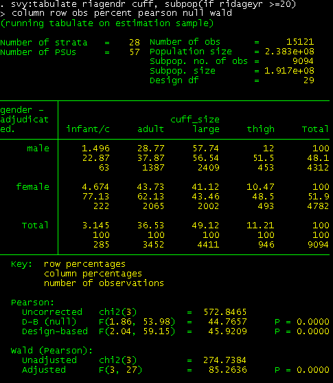
Use the svy : tabulate command to produce two-way tabulations for gender (riagendr) and blood pressure cuff size (cuff_size) with tests of independence for people age 20 years and older. (See Section 5.4 of Korn and Graubard Analysis of Data from Health Surveys, pp 207-211). Use the subpop( ) option to select a subpopulation for analysis, rather than select the study population in the Stata program while preparing the data file. This example uses an if statement to define the subpopulation based on the age variable's (ridageyr) value. Another option is to create a dichotomous variable where the subpopulation of interest is assigned a value of 1, and everyone else is assigned a value of 0. The options specified for this example, use the column, rows, obs, percent, pearson, null and wald test statistic options.
svy:tab riagendr cuff_size, subpop (if ridageyr >=20 & ridageyr<.) column row obs percent pearson null wald

Here is a table summarizing the output:
| Variable |
Men age 20 and older (n=4312) |
Women age 20 and older (n=4782) |
p value |
|---|---|---|---|
| Cuff size | |||
| (1) Infant | 0% | 0% | <0.0001 |
| (2) Child | 1.5% | 5% | |
| 3 Adult | 29% | 44% | |
| 4 Large | 58% | 41% | |
| 5 Thigh |
12% |
10% |
Men have a larger cuff size than women for example, 70% of men had cuff size of 4 or 5 compared to 51% of women. Cuff size varies significantly according to gender (p<0.0001). NOTE: The grayed cells have too few observations to create stable estimates and should probably not be reported.