Task 5: Key Concepts about Linear Regression
In cross-sectional surveys such as NHANES, linear regression analyses can be used to examine the association between multiple covariates and a health outcome measured on a continuous scale. For example, we will assess the association between systolic blood pressure (Y) and selected covariates (Xi) in this module. The covariates in this example will include calcium supplement use, race/ethnicity, age, and body mass index (BMI).
Simple linear regression is used when you have a single independent variable (e.g., supplement use); multiple linear regression may be used when you have more than one independent variable (e.g., supplement use and one or more covariates). Multiple regression allows you to examine the effect of the exposure of interest on the outcome after accounting for the effects of other variables (called covariates or confounders).
Simple linear regression is used to explore associations between one (continuous, ordinal or categorical) exposure and one (continuous) outcome variable. Simple linear regression lets you answer questions like, "How does systolic blood pressure vary with supplement use?".
Multiple linear regression is used to explore associations between two or more exposure variables (which may be continuous, ordinal or categorical) and one (continuous) outcome variable. The purpose of multiple linear regression is to isolate the relationship between the exposure variable and the outcome variable from the effects of one or more other variables called covariates. For example, say that systolic blood pressure values tend to be lower in younger people; and younger people are less likely to take calcium supplements. In this case, inferences about systolic blood pressure and calcium supplement use get confused by the effect of age on supplement use and blood pressure. This kind of "confusion" is called confounding (and these covariates are sometimes called confounders). Confounders are variables which are associated with both the exposure and outcome of interest. This relationship is shown in the following figure.
Diagram of the Relationship between Exposure, Outcome, and the Confounder
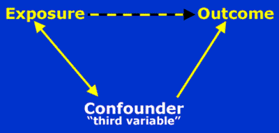
You can use multiple linear regression to adjust for confounding and isolate the relationship of interest. In this example, the relationship is between systolic blood pressure level and calcium supplement use. That is, multiple linear regression lets you answer the question, "How does systolic blood pressure vary with calcium supplement use, after accounting for — or unconfounded by — or independent of — age?" As mentioned, you can include many covariates at one time. The process of accounting for covariates is also called adjustment.
Comparing the results of simple and multiple linear regressions can help to answer the question "How much did the covariates in the model distort the relationship between exposure and outcome (i.e., how much confounding was there)?"
Note that getting statistical packages like SUDAAN, SAS Survey, and Stata to run analyses is the easy part of regression. What is not easy is knowing which variables to include in your analyses, how to represent them, when to worry about confounding, determining if your models are any good, and knowing how to interpret them. These tasks require thought, training, experience, and respect for the underlying assumptions of regression. Remember, garbage in - garbage out.
Finally, remember that NHANES analyses can only establish associations and not causal relationships. This is because the data are cross-sectional, so there is no way to establish temporal sequences (i.e., which came first the "exposure" or the "outcome"?).
This module will assess the association between systolic blood pressure (the continuous outcome variable) and selected covariates to show how to use linear regression with SUDAAN and SAS. The covariates in this example will include calcium supplement use, race/ethnicity, age, and body mass index (BMI). In other words, what is the effect of each of these variables, independent of the effect of the other variables?
Simple Linear Regression Model
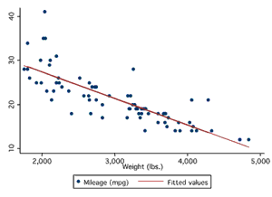
In the simplest case, you plot the values of a dependent, continuous variable Y against an independent, continuous variable X1, (i.e. a correlation) and see the best-fit line that can be drawn through the points.
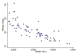
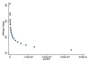
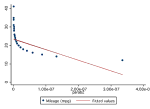
The first thing to do is make sure the relationship of interest is linear (since linear regression draws a straight line through data points). The best way to do this is to look at a scatterplot. If the relationship between variables is linear, continue (see panels A and B below). If it is not linear, do not use linear regression. In this case, you can try and transforming the data or using other forms of regression such as polynomial regression.
Example of a Linear Relationship
Panel A
Panel B
Example of a Non-linear Relationship
Panel C
Panel D
This relationship between X1 and Y can be expressed as
Equation for Simple Linear Regression
 (1)
(1)
b0 also known as the intercept, denotes the point at which the line intersects the vertical axis; b1 , or the slope, denotes the change in dependent variable, Y, per unit change in independent variable, X 1; and ε indicates the degree to which the plot of Y against X differs from a straight line. Note that for survey data, ε is always greater than 0.
Multiple Regression Model
You can further extend equation (1) to include any number of independent variables Xi , where i=1,..,n (both continuous (e.g. 0-100) and discrete (e.g. 0,1 or yes/no)).
Equation for Multiple Regression Model
![]() (2)
(2)
The choice of variables to include in equation (2) can be based on results of univariate analyses, where Xi and Y have a demonstrated association. It also can be based on empirical evidence where a definitive association between Y and an independent variable has been demonstrated in previous studies.
Polynomial Regression
It is possible to have two continuous variables, Y and X1, on sampled individuals such that if the values of Y are plotted against the values of X1, the resulting plot would resemble a parabola (i.e., the value of Y could increase with increasing values of X, level off and then decline). A polynomial regression model is used to describe this relationship between X1 and Y and is expressed as
Equation for Polynomial Regression
![]() (3)
(3)
Interaction
Consider the situation described in equation (2), where a discrete independent variable, X2, and a continuous independent variable, X1, affect a continuous dependent variable, Y. This relationship would yield two straight lines, one showing the relationship between Y and X1 for X2=0, and the other showing the relationship of Y and X1 for X2=1. If these straight lines were parallel, the rate of change of Y per unit change in X1 would be the same for X2=0 as for X2=1, and therefore, there would be no interaction between X1 and X2. If the two lines were not parallel, the relationship between Y and X1 would depend upon the relationship between Y and X2, and therefore there would be an interaction between X1 and X2.
Interpretation of Coefficients
For continuous independent variables, the beta coefficient indicates the change in the dependent variable per unit change in the independent variable, controlling for the confounding effects of the other independent variables in the model. A discrete random variable, X1, can assume 2 or more distinct values corresponding to the number of subgroups in a given category. One subgroup (usually arbitrarily) is designated as the reference group. The beta coefficient for a discrete variable indicates the difference in the dependent variable for one value of Xi (e.g., the difference between supplement users and the reference group, non-users), when all other independent variables in the model are held constant. A positive value for the beta coefficient indicates a larger value of the dependent variable for the subgroup (supplement users) than for the reference group (non-users), whereas a negative value for the beta coefficient indicates a smaller value.
:
| Independent variable type | Examples | What does the b coefficient mean in Simple linear regression? | What does the b coefficient mean in Multiple linear regression? |
|---|---|---|---|
| Continuous | height, weight, LDL | The change in the dependent variable per unit change in the independent variable. | The change in the dependent variable per unit change in the independent variable after controlling for the confounding effects of the covariates in the model. |
| Categorical | Supplement use (2 subgroups, users and non-users where one is designated as the reference group (non-users, in this example)). | The difference in the dependent variable for one value of categorical variable (e.g., the difference between supplement users and the reference group, non-users). | The difference in the dependent variable for one value of categorical variable (e.g., between supplement users and the reference group non-users), after controlling for the confounding effects of the covariates in the model. |
SUDAAN ((proc regress), SAS Survey (proc surveyreg), andStata (svy:regress) procedures produce beta coefficients, standard errors for these coefficients, confidence intervals, a t-statistic for the null hypothesis (i.e., ß=0), a p-value for the t-statistic (i.e., the probability of obtaining a value greater than or equal to the value for the t statistic).
![]() Close Window
to return to module page.
Close Window
to return to module page.